Dive into grid2op sequential decision process
This page is organized as follow:
Objectives
The goal of this page of the documentation is to provide you with a relatively extensive description of the mathematical model behind grid2op.
Grid2op is a software whose aim is to make experiments on powergrid, mainly sequential decision making, as easy as possible.
We chose to model this sequential decision making probleme as a “Markov Decision Process” (MDP) and one some cases “Partially Observable Markov Decision Process” (POMDP) or “Constrainted Markov Decision Process” (CMDP) and (work in progress) even “Decentralized (Partially Observable) Markov Decision Process” (Dec-(PO)MDP).
General notations
There are different ways to define an MDP. In this paragraph we introduce the notations that we will use.
In an MDP an “agent” / “automaton” / “algorithm” / “policy” takes some action  . This
action is processed by the environment and update its internal state from
. This
action is processed by the environment and update its internal state from  to
to  and
computes a so-called reward
and
computes a so-called reward ![r_{t+1} \in [0, 1]](_images/math/2f723c552706807ba297fda80793790768e33469.png) .
.
Note
By stating the dynamic of the environment this way, we ensure the “Markovian” property: the
state  is determined by the knowledge of the previous state
  and the
action
and the
action 
This tuple
 is then given to the “agent” / “automaton” / “algorithm” which in turns produce the action
Note
More formally even, everything written can be stochastic:
 where
where  is the “policy” parametrized by
some parameters
is the “policy” parametrized by
some parameters  that outputs here a probability distribution (depending on the
state of the environment
that outputs here a probability distribution (depending on the
state of the environment  ) over all the actions mathcal{A}
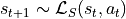 where
where  is a probability distribution
over
is a probability distribution
over  representing the likelyhood if the “next state” given the current state and the action
of the “policy”
representing the likelyhood if the “next state” given the current state and the action
of the “policy”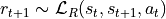 is the reward function indicating “how good”
was the transition from to by taking action
is the reward function indicating “how good”
was the transition from to by taking action 
This alternation  is done for a certain number of “steps” called
  .
.
We will call the list  an “episode”.
Formally the knowledge of:
- , the “state space”
 , the “action space”
 , sometimes called “transition kernel”, is the probability
distribution (over ) that gives the next
state after taking action
, sometimes called “transition kernel”, is the probability
distribution (over ) that gives the next
state after taking action  in state
 , sometimes called “reward kernel”,
is the probability distribution (over
, sometimes called “reward kernel”,
is the probability distribution (over ![[0, 1]](_images/math/8027137b3073a7f5ca4e45ba2d030dcff154eca4.png) ) that gives
the reward
) that gives
the reward  after taking action in state which lead to state
 the maximum number of steps for an episode
Defines a MDP. We will detail all of them in the section Modeling sequential decisions bellow.
In grid2op, there is a special case where a grid state cannot be computed (either due to some physical infeasibilities
or because the resulting state would be irrealistic). This can be modeled relatively easily in the MDP formulation
above if we add a “terminal state”  in the state space
 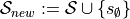 : and add the transitions:
 stating that once the agent lands in this “terminal state” then the game is over, it stays there until the
end of the scenario.
stating that once the agent lands in this “terminal state” then the game is over, it stays there until the
end of the scenario.
We can also define the reward kernel in this state, for example with
 and
and
 which
states that there is nothing to be gained in being in this terminal set.
which
states that there is nothing to be gained in being in this terminal set.
Unless specified otherwise, we will not enter these details in the following explanation and take it as
“pre requisite” as it can be defined in general. We will focus on the definition of ,
, and by leaving out the
“terminal state”.
Note
In grid2op implementation, this “terminal state” is not directly implemented. Instead, the first Observation leading to this state is marked as “done” (flag obs.done is set to True).
No other “observation” will be given by grid2op after an observation with obs.done set to True and the environment needs to be “reset”.
This is consistent with the gymnasium implementation.
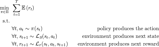
The main goal of a finite horizon MDP is then to find a policy  that given states and reward
output an action such that (NB here
that given states and reward
output an action such that (NB here  denotes the set of all considered policies for this
MDP):
denotes the set of all considered policies for this
MDP):
Specific notations
To define “the” MDP modeled by grid2op, we also need to define some other concepts that will be used to define the
state space or transition kernel for example.
A Simulator
We need a so called “simulator”.
Informatically, this is represented by the Backend inside the grid2op environment (more information about the Backend is detailed in the Backend section of the documentation).
This simulator is able to compute some informations that are part of the state
space (eg flows on powerlines, active production value of generators etc.)
and thus are used in the computation of the transition kernel.
We can model this simulator with a function  that takes as input some data from an
“input space”
that takes as input some data from an
“input space”  and result
in data in
and result
in data in  .
.
Note
In grid2op we don’t force the “shape” of , including
the format used to read the grid file from the hard drive, the solved equations, the way
these equations are used. Everything here is “free” and grid2op only needs that the simulator
(wrapped in a Backend) understands the “format” sent by grid2op (through a
grid2op.Action._backendAction._BackendAction) and is able to expose
to grid2op some of its internal variables (accessed with the ***_infos() methods of the backend)
TODO do I emphasize that the simulator also contains the grid iteself ?
To make a parallel with similar concepts “simulator”, represents the physics as in all “mujoco” environments eg Ant or Inverted Pendulum . This is the same concept here excepts that it solves powerflows.
Some Time Series
Another type of data that we need to define “the” grid2op MDP is the “time series”, implemented in the chronics grid2op module documented on the page Time series (formerly called “chronics”) with some complements given in the Input data of an environment page as well.
These time series define what exactly would happen if the grid was a “copper plate” without any constraints. Said differently it provides what would each consumer consume and what would each producer produce if they could all be connected together with infinite “bandwith”, without any constraints on the powerline etc.
In particular, grid2op supposes that these “time series” are balanced, in the sense that the producers produce just the right amount (electrical power cannot really be stocked) for the consumer to consume and that for each steps. It also supposes that all the “constraints” of the producers.
These time series are typically generated outside of grid2op, for example using chronix2grid python package (or anything else).
Formally, we will define these time series as input  all these time series at time
  . These
exogenous data consist of :
. These
exogenous data consist of :
generator active production (in MW), for each generator
load active power consumption (in MW), for each loads
load reactive consumption (in MVAr), for each loads
* generator voltage setpoint / target (in kV)
Note
* for this last part, this can be adapted “on demand” by the environment through the voltage controler module. But for the sake of modeling, this can be modeled as being external / exogenous data.
And, to make a parrallel with similar concept in other RL environment, these “time series” can represent the layout of the maze in pacman, the positions of the platforms in “mario-like” 2d games, the different turns and the width of the route in a car game etc. This is the “base” of the levels in most games.
Finally, for most released environment, a lof of different  are available. By default, each time the
environment is “reset” (the user want to move to the next scenario), a new is used (this behaviour
can be changed, more information on the section Time series Customization of the documentation).
are available. By default, each time the
environment is “reset” (the user want to move to the next scenario), a new is used (this behaviour
can be changed, more information on the section Time series Customization of the documentation).
Modeling sequential decisions
As we said in introduction of this page, we will model a given scenario in grid2op. We have at our disposal:
a simulator, which is represented as a function
some time series
In order to define the MDP we need to define:
- , the “state space”
- , the “action space”
- , sometimes called “transition kernel”, is the probability
distribution (over ) that gives the next
state after taking action in state
- , sometimes called “reward kernel”,
is the probability distribution (over ) that gives
the reward after taking action in state which lead to state
We will do that for a single episode (all episodes follow the same process)
Precisions
To make the reading of this MDP easier, for this section of the documentation, we adopted the following convention:
text in green will refer to elements that are read directly from the grid by the simulator
at the creation of the environment.text in orange will refer to elements that are related to time series
text in blue will refer to elements that can be be informatically modified by the user at the creation of the environment.
In the pure definition of the MDP all text in green, orange or blue are exogenous and constant: once the episode starts they cannot be changed by anything (including the agent).
We differenciate between these 3 types of “variables” only to clarify what can be modified by “who”:
green variables depend only on the controlled powergrid
orange variables depend only time series
blue variables depend only on the way the environment is loaded
Note
Not all these variables are independant though. If there are for example 3 loads on the grid, then you need to use time series that somehow can generate 3 values at each step for load active values and 3 values at each step for load reactive values. So the dimension of the orange variables is somehow related to dimension of green variables : you cannot use the time series you want on the grid you want.
Structural informations
To define mathematically the MPD we need first to define some notations about the grid manipulated in this episode.
We suppose that the structure of the grid does not change during the episode, with:
n_line being the number of “powerlines” (and transformers) which are elements that allow the power flows to actually move from one place to another
n_gen being the number of generators, which are elements that produces the power
n_load being the number of consumers, which are elements that consume the power (typically a city or a large industrial plant manufacturing)
n_storage being the number of storage units on the grid, which are elements that allow to convert the power into a form of energy that can be stored (eg chemical)
All these elements (side of powerlines, generators, loads and storage units) are connected together at so called “substation”. The grid counts n_sub such substations. We will call dim_topo := 2 times n_line + n_gen + n_load + n_storage the total number of elements in the grid.
Note
This “substation” concept only means that if two elements does not belong to the same substations, they cannot be directly connected at the same “node” of the graph.
They can be connected in the same “connex component” of the graph (meaning that there are edges that can connect them) but they cannot be part of the same “node”
Each substation can be divided into n_busbar_per_sub (was only 2 in grid2op <= 1.9.8 and can be any integer > 0 in grid2op version >= 1.9.9).
This n_busbar_per_sub parameters tell the maximum number of independant nodes their can be in a given substation.
So to count the total maximum number of nodes in the grid, you can do

When the grid is loaded, the backend also informs the environment about the ***_to_subid vectors (eg gen_to_subid) which give, for each element to which substation they are connected. This is how the “constraint” of
Note
Definition
With these notations, two elements are connected together if (and only if, that’s a definition after all):
they belong to the same substation
they are connected to the same busbar
In this case, we can also say that these two elements are connected to the same “bus”.
These “buses” are the “nodes” in “the” graph you thought about when looking at a powergrid.
Note
Definition (“disconnected bus”): A bus is said to be disconnected if there are no elements connected to it.
Note
Definition (“disconnected element”): An element (side of powerlines, generators, loads or storage units) is said to be disconnected if it is not connected to anything.
Extra references:
You can modify n_busbar_per_sub in the grid2op.make function. For example, by default if you call grid2op.make(“l2rpn_case14_sandbox”) you will have n_busbar_per_sub = 2 but if you call grid2op.make(“l2rpn_case14_sandbox”, n_busbar=3) you will have n_busbar_per_sub = 3 see Substations for more information.
n_line, n_gen, n_load, n_storage and n_sub depends on the environment you loaded when calling grid2op.make, for example calling grid2op.make(“l2rpn_case14_sandbox”) will lead to environment with n_line = 20, n_gen = 6, n_load = 11 and n_storage = 0.
Other informations
When loading the environment, there are also some other static data that are loaded which includes:
min_storage_p and max_storage_p: the minimum power that can be injected by each storage units (typically min_storage_p
 ). These are vectors
(of real numbers) of size n_storage
). These are vectors
(of real numbers) of size n_storageis_gen_renewable: a vector of True / False indicating for each generator whether it comes from new renewable (and intermittent) renewable energy sources (eg solar or wind)
is_gen_controlable: a vector of True / False indicating for each generator whether it can be controlled by the agent to produce both more or less power at any given step. This is usually the case for generator which uses as primary energy coal, gaz, nuclear or water (hyrdo powerplant)
min_ramp and max_ramp: are two vector giving the maximum amount of power each generator can be adjusted to produce more / less. Typically, min_ramp = max_ramp = 0 for non controlable generators.
Note
These elements are marked green because they are loaded by the backend, but strictly speaking they can be specified in other files than the one representing the powergrid.
Action space
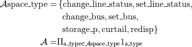
At time of writing, grid2op support different type of actions:
change_line_status: that will change the line status (if it is disconnected this action will attempt to connect it). It leaves in

set_line_status: that will set the line status to a particular state regardless of the previous state (+1 to attempt a force reconnection on the powerline and -1 to attempt a force disconnection). There is also a special case where the agent do not want to modify a given line and it can then output “0” It leaves in
* change_bus: that will, for each element of the grid change the busbars to which it is connected (eg if it was connected on busbar 1 it will attempt to connect it on busbar 2). This leaves in

set_bus: that will, for each element control on which busbars you want to assign it to (1, 2, …, n_busbar_per_sub). To which has been added 2 special cases -1 means “disconnect” this element and 0 means “I don’t want to affect” this element. This part of the action space then leaves in

storage_p: for each storage, the agent can chose the setpoint / target power for each storage units. It leaves in
![[\text{min\_storage\_p}, \text{max\_storage\_p}] \subset \mathbb{R}^{\text{n\_storage}}](_images/math/5ff633385d35353b2ecebe455b0da6e0d37c5f6c.png)
curtail: corresponds to the action where the agent ask a generator (using renewable energy sources) to produce less than what would be possible given the current weather. This type of action can only be performed on renewable generators. It leaves in
![[0, 1]^{\text{n\_gen}}](_images/math/1f5d9fb1834f1461b7f3458f97ba2c6816270c81.png) (to avoid getting the notations even more complex, we won’t define exactly the space of this
action. Indeed, writing is not entirely true as a non renewable generator
will not be affected by this type of action)
(to avoid getting the notations even more complex, we won’t define exactly the space of this
action. Indeed, writing is not entirely true as a non renewable generator
will not be affected by this type of action)redisp: corresponds to the action where the agent is able to modify (to increase or decrease) the generator output values (asking at the some producers to produce more and at some to produce less). It leaves in
![[\text{min\_ramp}, \text{max\_ramp}] \subset \mathbb{R}^{\text{n\_gen}}](_images/math/f0a9c82def68c692470868993dadab8efbfd1c2e.png) (remember that for non controlable generators, by definition we suppose that min_ramp = max_ramp = 0)
(remember that for non controlable generators, by definition we suppose that min_ramp = max_ramp = 0)
Note
The change_bus is only available in environment where n_busbar_per_sub = 2 otherwise this would not make sense. The action space does not include this type of actions if n_busbar_per_sub != 2
You might have noticed that every type of actions is written in blue. This is because the action space can be defined at the creation of the environment, by specifying in the call to grid2op.make the action_class to be used.
Let’s call  either
(corresponding to the definition of the change_line_status briefly described above) if the
change_line_status has been selected by the user (for the entire scenario) or the
either
(corresponding to the definition of the change_line_status briefly described above) if the
change_line_status has been selected by the user (for the entire scenario) or the
 otherwise (and we do similarly for all other type of actions of course: for example:
![1_{redisp} \in \left\{[\text{min\_ramp}, \text{max\_ramp}], \emptyset\right\}](_images/math/a92b1828538d17324945c8423efdc6222964a071.png) )
)
Formally then, the action space can then be defined as:
Note
In the grid2op documentation, the words “topological modification” are often used. When that is the case, unless told otherwise it means set_bus or change_bus type of actions.
Extra references:
Informatically, the can be define at the
call to grid2op.make when the environment is created (and cannot be changed afterwards).
For example, if the user build the environment like this :
import grid2op
from grid2op.Action import PlayableAction
env_name = ... # whatever, eg "l2rpn_case14_sandbox"
env = grid2op.make(env_name, action_class=PlayableAction)
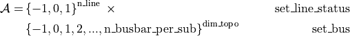
Then all type of actions are selected and :
![\begin{align*}
\mathcal{A} =& \left\{0,1\right\}^{\text{n\_line}}~ \times & \text{change\_line\_status} \\
& \left\{-1, 0, 1\right\}^{\text{n\_line}}~ \times & \text{set\_line\_status} \\
& \left\{0,1\right\}^{\text{dim\_topo}}~ \times & \text{change\_bus} \\
& \left\{-1, 0, 1, 2, ..., \text{n\_busbar\_per\_sub} \right\}^{\text{dim\_topo}}~ \times & \text{set\_bus} \\
& ~[\text{min\_storage\_p}, \text{max\_storage\_p}]~ \times & \text{storage\_p} \\
& ~[0, 1]^{\text{n\_gen}} \times & \text{curtail} \\
& ~[\text{min\_ramp}, \text{max\_ramp}] & \text{redisp}
\end{align*}](_images/math/4229d51a24d7a811b74790f70b093cf636e7e48d.png)
You can also build the same environment like this:
import grid2op
from grid2op.Action import TopologySetAction
same_env_name = ... # whatever, eg "l2rpn_case14_sandbox"
env = grid2op.make(same_env_name, action_class=TopologySetAction)
Which will lead the following action space, because the user ask to use only “topological actions” (including line status) with only the “set” way of modifying them.
The page Action of the documentation provides you with all types of actions you you can use in grid2op.
Note
If you use a compatibility with the popular gymnasium (previously gym) you can also specify the action space with the “attr_to_keep” key-word argument.
State space
By default in grid2op, the state space shown to the agent (the so called “observation”). In this part of the documentation, we will described something slightly different which is the “state space” of the MDP.
The main difference is that this “state space” will include future data about the
environment (eg the matrix). You can refer to
section Partial Observatibility or Or not partial observatibility ? of this page of the documentation.
Note
We found it easier to show the MDP without the introduction of the “observation kernel”, so keep in mind that this paragraph is not representative of the observation in grid2op but is “purely theoretical”.
The state space is defined by different type of attributes and we will not list them all here (you can find a detailed list of everything available to the agent in the Observation page of the documentation.) The “state space” is then made of:
some part of the outcome of the solver:
 , this
includes but is not limited to the loads active values load_p,
loads reactive values load_q, voltage magnitude
at each loads load_v, the same kind of attributes but for generators
gen_p, gen_q, gen_v, gen_theta and also for powerlines
p_or, q_or, v_or, a_or, theta_or, p_ex, q_ex, v_ex,
a_ex, theta_ex, rho etc.
, this
includes but is not limited to the loads active values load_p,
loads reactive values load_q, voltage magnitude
at each loads load_v, the same kind of attributes but for generators
gen_p, gen_q, gen_v, gen_theta and also for powerlines
p_or, q_or, v_or, a_or, theta_or, p_ex, q_ex, v_ex,
a_ex, theta_ex, rho etc.some attributes related to “redispatching” (which is a type of actions) that is computed by the environment (see Transition Kernel for more information) which includes target_dispatch and actual_dispatch or the curtailment gen_p_before_curtail, curtailment_mw, curtailment or curtailment_limit
some attributes related to “storage units”, for example storage_charge , storage_power_target, storage_power or storage_theta
some related to “date” and “time”, year, month, day, hour_of_day, minute_of_hour, day_of_week, current_step, max_step, delta_time
finally some related to the rules of the game like timestep_overflow, time_before_cooldown_line or time_before_cooldown_sub
And, to make it “Markovian” we also need to include :
the (constant) values of
that
are not “part of” (more information about that in
the paragraph “Step 4: Call the simulator” of this documentation).
This might include some physical
parameters of some elements of the grid (like transformers or powerlines) or
some other parameters of the solver controlling either the equations to be
solved or the solver to use etc. *the complete matrix
which include the exact knowledge of
past, present and future loads and generation for the entire scenario (which
is not possible in practice). The matrix itself is constant.the index representing at which “step” of the matrix
the
current data are being used by the environment.
Note
* grid2op is build to be “simulator agnostic” so all this part of the “state space”
is not easily accessible through the grid2op API. To access (or to modify) them
you need to be aware of the implementation of the grid2op.Backend.Backend
you are using.
Note
In this modeling, by design, the agent sees everything that will happen in the future, without uncertainties. To make a parrallel with a “maze” environment, the agent would see the full maze and its position at each step.
This is of course not fully representative of the daily powergrid operations, where the operators cannot see exactly the future. To make this modeling closer to the reality, you can refer to the paragphs Partial Observatibility and Or not partial observatibility ? below.
Transition Kernel
In this subsection we will describe the so called transition kernel, this is the function that given a
state and an action gives a probability distribution over all possible next state
 .
.
In this subsection, we chose to model this transition kernel as a deterministic
function (which is equivalent to saying that the probability distribution overs is
a Dirac distribution).
Note
The removal of the matrix in the “observation space” see section Partial Observatibility or the
rewriting of the MDP to say in the “fully observable setting” (see section Or not partial observatibility ?) or the
introduction of the “opponent” described in section Adversarial attacks are all things that “makes” this
“transition kernel” probabilistic. We chose the simplicity in presenting it in a fully deterministic
fashion.
So let’s write what the next state is given the current state  and the action of
the agent
and the action of
the agent  . To do that we split the computation in different steps explained bellow.
Note
To be exhaustive, if the actual state is  then the
  is
returned regardless of the action and the steps described below are skipped.
is
returned regardless of the action and the steps described below are skipped.
If the end of the episode is reached then is returned.
Step 1: legal vs illegal
The first step is to check if the action is legal or not. This depends on the rules (see the dedicated page Rules of the Game of the documentation) and the parameters (more information at the page Parameters of the documentation). There are basically two cases:
the action
is legal: then proceed to next stepthe action
is not, then replace the action by do nothing, an action that does not
affect anything and proceed to next step
Step 2: load next environment values
This is also rather straightforward, the current index is updated (+1 is added) and this
new index is used to find the “optimal” (from a market or a central authority perspective)
value each producer produce to satisfy the demand mof each consumers (in this case large cities or
companies). These informations are stored in the matrix.
Step 3: Compute the generators setpoints and handle storage units
The next step of the environment is to handle the “continuous” part of the action (eg “storage_p”, “curtail” or “redisp”) and to make sure a suitable setpoint can be reached for each generators (you can refer to the pages Storage units (optional) and Generators of this documentation for more information).
There are two alternatives:
either the physical constraints cannot be met (there exist no feasible solutions for at least one generator), and in this case the next state is the terminal state
(ignore all the steps bellow)or they can be met. In this case the “target generator values” is computed as well as the “target storage unit values”
Note
There is a parameters called LIMIT_INFEASIBLE_CURTAILMENT_STORAGE_ACTION that will
try to avoid, as best as possible to fall into infeasibile solution. It does so by limiting
the amount of power that is curtailed or injected in the grid from the storage units: it
modifies the actions .
Step 4: Call the simulator
At this stage then (assuming the physical constraints can be met), the setpoint for the following variables is known:
the status of the lines is deduced from the “change_line_status” and “set_line_status” and their status in
(the current state). If there are maintenance (or attacks, see section
Adversarial attacks) they can also disconnect powerlines.the busbar to which each elements is connected is also decuced from the “change_bus” and “set_bus” part of the action
the consumption active and reactive values have been computed from the
values at previous stepthe generator active values have just been computed after taking into account the redispatching, curtailement and storage (at this step)
the voltage setpoint for each generators is either read from
or
deduced from the above data by the “voltage controler” (more information on Voltage Controler)
All this should be part of the input solver data . If not, then the
solver cannot be used unfortunately…
With that (and the other data used by the solver and included in the space, see paragraph
State space of this documentation), the necessary data is shaped (by the Backend) into
a valid  .
.
The solver is then called and there are 2 alternatives (again):
either the solver cannot find a feasible solution (it “diverges”), and in this case the next state is the terminal state
(ignore all the steps bellow)or a physical solution is found and the process carries out in the next steps
Step 5: Emulation of the “protections”
At this stage an object  has been computed by the solver.
The first step performed by grid2op is to look at the flows (in Amps) on the powerlines (these data
are part of  ) and to check whether they meet some constraints
defined in the parameters (mainly if for some powerline the flow is too high, or if it has been
too high for too long, see HARD_OVERFLOW_THRESHOLD, NB_TIMESTEP_OVERFLOW_ALLOWED and
NO_OVERFLOW_DISCONNECTION). If some powerlines are disconnected at this step, then the
“setpoint” send to the backend at the previous step is modified and it goes back
to Step 4: Call the simulator.
) and to check whether they meet some constraints
defined in the parameters (mainly if for some powerline the flow is too high, or if it has been
too high for too long, see HARD_OVERFLOW_THRESHOLD, NB_TIMESTEP_OVERFLOW_ALLOWED and
NO_OVERFLOW_DISCONNECTION). If some powerlines are disconnected at this step, then the
“setpoint” send to the backend at the previous step is modified and it goes back
to Step 4: Call the simulator.
Note
The simulator can already handle a real simulation of these “protections”. This “outer loop” is because some simulators does not do it.
Note
For the purist, this “outer loop” necessarily terminates. It is trigger when at least one powerline needs to be disconnected. And there are n_line (finite) powerlines.
Step 6: Reading back the “grid dependant” attributes
At this stage an object
has been computed by the solver and all the “rules” / “parameters” regarding powerlines
are met.
As discussed in the section about “state space” (see State space for more information),
the next state space include some part of the outcome of the solver. These data
are then read from the , which
includes but is not limited to the loads active values load_p,
loads reactive values load_q, voltage magnitude
at each loads load_v, the same kind of attributes but for generators
gen_p, gen_q, gen_v, gen_theta and also for powerlines
p_or, q_or, v_or, a_or, theta_or, p_ex, q_ex, v_ex,
a_ex, theta_ex, rho etc.
Step 7: update the other attributes of the state space
Finally, the environment takes care of updating all the other “part” of the state space, which are:
attributes related to “redispatching” are updated at in paragraph Step 3: Compute the generators setpoints and handle storage units
and so are attributes related to storage units
the information about the date and time are loaded from the
matrix.
As for the attributes related to the rules of the game, they are updated in the following way:
timestep_overflow is set to 0 for all powerlines not in overflow and increased by 1 for all the other
time_before_cooldown_line is reduced by 1 for all line that has not been impacted by the action
otherwise set to param.NB_TIMESTEP_COOLDOWN_LINEtime_before_cooldown_sub is reduced by 1 for all substations that has not been impacted by the action
otherwise set to param.NB_TIMESTEP_COOLDOWN_SUB
The new state is then passed to the agent.
Note
We remind that this process might have terminated before reaching the last step described above, for example at Step 3: Compute the generators setpoints and handle storage units or at Step 4: Call the simulator or during the emulation of the protections described at Step 5: Emulation of the “protections”
Reward Kernel
And to finish this (rather long) description of grid2op’s MDP we need to mention the “reward kernel”.
This “kernel” computes the reward associated to taking the action in step
that lead to step . In most cases, the
reward in grid2op is a deterministic function and depends only on the grid state.
In grid2op, every environment comes with a pre-defined reward function that can be fully customized by the user when the environment is created or even afterwards (but is still constant during an entire episode of course).
For more information, you might want to have a look at the Reward page of this documentation.
Extensions
In this last section of this page of the documentation, we dive more onto some aspect of the grid2op MDP.
Note
TODO: This part of the section is still an ongoing work.
Let us know if you want to contribute !
Partial Observatibility
This is the case in most grid2op environments: only some part of the environment
state at time t are
given to the agent in the observation at time t  .
.
Mathematically this can be modeled with the introduction of an “observation space” and an
“observation kernel”. This kernel will only expose part of the “state space” to the agent and
(in grid2op) is a deterministic function that depends on the environment state .
More specifically, in most grid2op environment (by default at least), none of the
physical parameters of the solvers are provided. Also, to represent better
the daily operation in power systems, only the t th row of the matrix
is given in the observation . The components  (for
(for  ) are not given. The observation kernel in grid2op will
mask out some part of the “environment state” to the agent.
) are not given. The observation kernel in grid2op will
mask out some part of the “environment state” to the agent.
Or not partial observatibility ?
If we consider that the agent is aware of the simulator used and all it’s “constant” (see
paragraph State space) part of
(which are part of the simulator that are not affected by the actions of
the agent nor by environment) then we can model the grid2op MDP without the need
to use an observation kernel: it can be a regular MDP.
To “remove” the need of partial observatibility, without the need to suppose that the
agent sees all the future we can adapt slightly the modeling which allows us to
remove completely the matrix :
the observation space / state space (which are equal in this setting) are the same as the one used in Partial Observatibility
the transition kernel is now stochastic. Indeed, the “next” value of the loads and generators are, in this modeling not read from a
matrix but sampled from a given
distribution which replaces the step Step 2: load next environment values of subsection
Transition Kernel. And once the values of these variables are sampled,
the rest of the steps described there are unchanged.
Note
The above holds as long as there exist a way to sample new values for gen_p, load_p, gen_v and load_q that is markovian. We suppose it exists here and will not write it down.
Note
Sampling from these distribution can be quite challenging and will not be covered here.
One of the challenging part is that the sampled generations need to meet the demand (and the losses) as well as all the constraints on the generators (p_min, p_max and ramps)
Adversarial attacks
TODO: explain the model of the environment
Forecast and simulation on future states
TODO : explain the model the forecast and the fact that the “observation” also includes a model of the world that can be different from the grid of the environment
Simulator dynamics can be more complex
TODO, Backend does not need to “exactly map the simulator” there are some examples below:
Hide elements from the grid2op environment
TODO only a part of the grid would be “exposed” in the grid2op environment.
Contain elements not modeled by grid2op
TODO: speak about HVDC or “pq” generators, or 3 winding transformers
Contain embeded controls
TODO for example automatic setpoint for HVDC or limit on Q for generators
Time domain simulation
TODO: we can plug in simulator that solves more accurate description of the grid and only “subsample” (eg at a frequency of every 5 mins) provide grid2op with some information.
Handle the topology differently
Backend can operate switches, only requirement from grid2op is to map the topology to switches.
Some constraints
TODO
Operator attention: alarm and alter
TODO
If you still can’t find what you’re looking for, try in one of the following pages:
Still trouble finding the information ? Do not hesitate to send a github issue about the documentation at this link: Documentation issue template
Copyright © Grid2Op a Series of LF Projects, LLC For website terms of use, trademark policy and other project policies please see https://lfprojects.org.